Bathymetric Data Wrangling

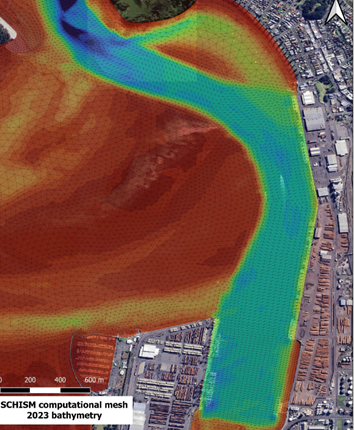
Figure 1: Detailed bathymetry near the Port of Tauranga served as one of many inputs to a SCHISM hydrodynamic model.

While all of Earth’s land surfaces have been mapped at 30 m resolution or finer, the topography of the seabed is still largely a black box, with only 26.1% of the seabed mapped to “adequate resolution” thus far. At MetOcean, we run a variety of wave and hydrodynamic models which require detailed information about the ocean’s depths in the form of a Digital Elevation Model (DEM), a continuous, gridded map of the sea floor over the model domain. Compiling such a bathymetric dataset often involves “filling in” areas of missing data, “smoothing” conflicts between overlapping datasets, and “blending” information from multiple sources.

What is bathymetry and how is it measured?

Bathymetry refers to “submarine topography”, e.g. the depths and shapes of underwater terrain. A bathymetric map is like an inverted topo map, with elevations measured below, rather than above, some zero baseline, such as mean sea level. The earliest bathymetric maps were based on sparse point measurements taken via line and sinker. Nowadays, high resolution, synoptic scale bathymetry is achieved via multibeam echosounding (MBES). MBES involves emitting a fan of acoustic waves from a boat mounted sensor and inferring the water depths based on the time it takes the signal to bounce off the sea floor and return to the sensor. Though MBES can achieve submeter-scale accuracy and near-complete coverage of the surveyed area, such surveys are expensive to conduct and infeasible in unnavigable areas such as the surf and coastal zones. As a result, only a small fraction of the ocean has been mapped with MBES, so we continue to rely on a multitude of lower resolution, sparse, indirect or interpolated measurements to fill in the gaps.

Challenges working with bathymetry data

Bathymetric data comes in many forms, ranging from chart data, survey transects, MBES, topographic data of land features, and the coarse resolution global GEBCO grid. With the general goal being to compile the most up-to-date, detailed and accurate bathymetry over the model area of interest, multiple data sources must often be combined and reconciled. Two common challenges arise: one is data fusion, which refers to the merging of overlapping or adjacent datasets; the other is interpolation, which encompasses techniques used to fill in gaps where no adequate data exists.

Fusion

Perhaps the simplest method of data fusion is “data stacking” where higher priority data is overlaid on top of lower priority data, perhaps due to the former’s superior resolution, accuracy, or recent acquisition. Data stacking often produces “edge effects” where there is a noticeable seamline at the edge of overlap due to disparities between the datasets. One solution for mitigating this artificial edge is “weighted blending,” proposed by Petrasova et al 2017. The method assumes a higher quality model with less coverage (DEM A) and a lower quality model with more coverage (DEM B). The elevation values covered by DEM A are prioritized over all areas that it covers except within a “buffer zone” along the edge where the two DEMs overlap. The width of the buffer zone is spatially varying based on how different the two DEMs are along the edge. Within this buffer zone, the elevation values from both DEMs are considered and weighted according to how far from edges of each DEM they are.

This method is illustrated for a small island in the Bay of Plenty using a 25 m combined bathy/topo dataset and a 1 m lidar dataset covering the land area only. The difference between simply stacking the two models on top of each other versus weighted blending is quite apparent.

Interpolation

Numerous interpolation methods have been developed to fill gaps between data points. The underlying assumption of interpolation is Tobler’s first law of geography: “everything is related to everything else, but near things are more related than distant things.” Interpolation methods infer values at unsurveyed locations using information from nearby observations via strategies such as:

-            Nearest neighbour: Assign the interpolation point the same value as the closest observation

-            Linear and spline: Fit a mathematically defined line or curve through nearby observations and derive interpolation values from the function

-            Inverse distance weighting: Take a weighted average of nearby observations, with closer ones having more weight than further ones

-            Kriging: Model the statistical properties of observations and use that model to derive the point value

When interpolating bathymetry data, these methods can produce quite variable results as shown in the interpolation of navigation chart point depths and contours below compared with high resolution MBES data over the same area.

Ellorine Carle